Data Blog
Data Science, Machine Learning and Statistics, implemented in Python
AB Testing: effect of early peeking and what to do about it
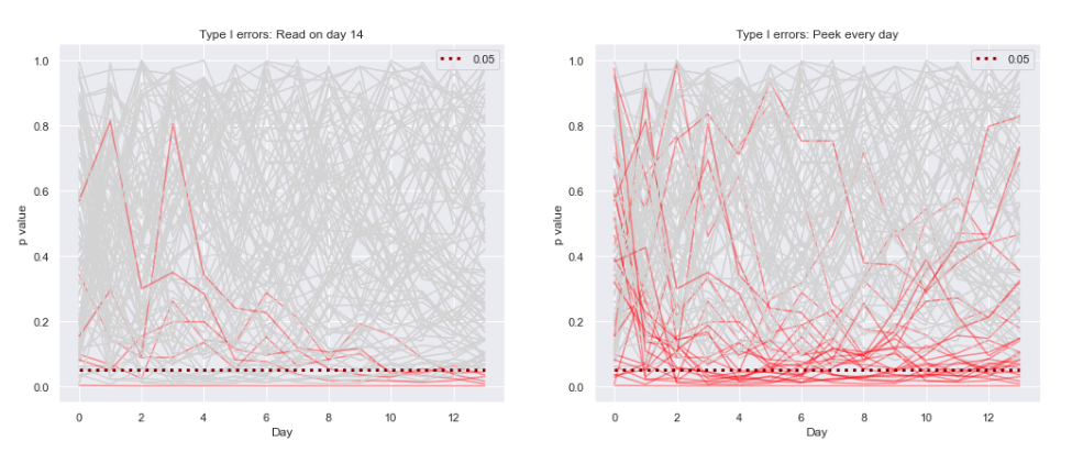
— Xavier Bourret SicotteThis notebook simulates the impact of early peaking on the results of a conversion rate AB test. Early peaking is loosely defined as the practice of checking and concluding the results of an AB test (i.e. based on its p value, statistical significance, secondary metrics etc) before the target sample size and power are reached.
 Tags:
Tags:
Comparing t-test and Mann Whitney test for the means of Gamma
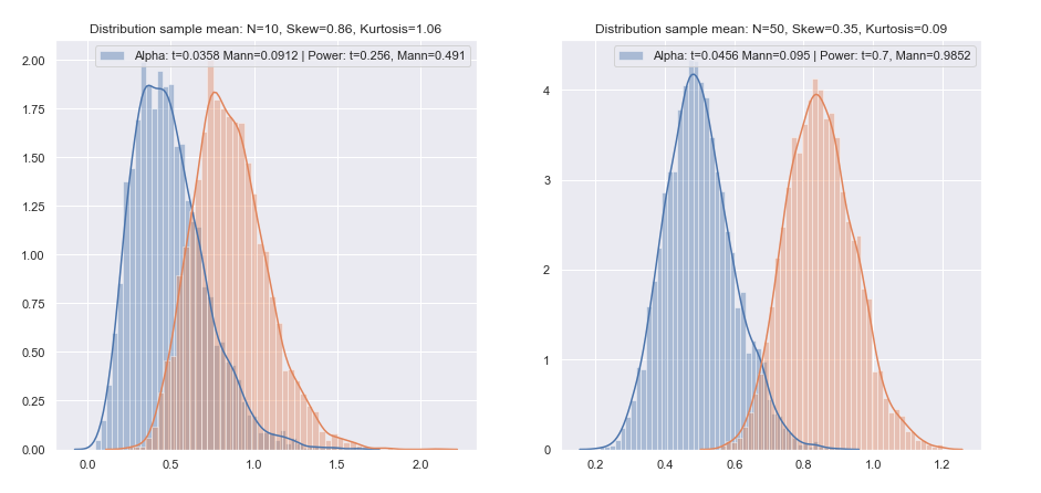
— Xavier Bourret SicotteThis notebook explores various simulations where we are testing for the difference in means of two independent gamma distributions, by sampling them and computing the means of each sample. We will compare two main test methods: the t-test and the Mann Whitney test.
 Tags:
Tags:
Gaussian Mixture Model EM Algorithm - Vectorized implementation
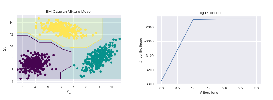
— Xavier Bourret SicotteImplementation of a Gaussian Mixture Model using the Expectation Maximization Algorithm. Vectorized implementation using Python Numpy and comparison to the Sklearn implementation on a toy data set
 Tags:
Tags:
AdaBoost: Implementation and intuition
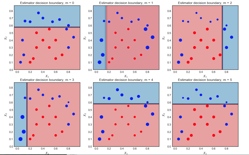
— Xavier Bourret SicotteThis notebook explores the well known AdaBoost M1 algorithm which combines several weak classifiers to create a better overall classifier. The notebook consists of three main sections: A review of the Adaboost M1 algorithm and an intuitive visualization of its inner workings. An implementation from scratch in Python, using an Sklearn decision tree stump as the weak classifier. A discussion on the trade-off between the Learning rate and Number of weak classifiers parameters
 Tags:
Tags:
Tree based models
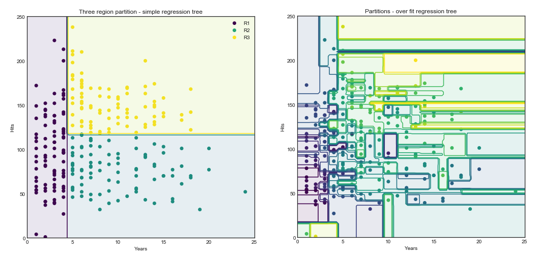
— Xavier Bourret SicotteThis notebook explores chapter 8 of the book "Introduction to Statistical Learning" and aims to reproduce several of the key figures and discussion topics. Of interest is the use of the graphviz library to help visualize the resulting trees and GridSearch from the Sklearn library to plot the validation curves
 Tags:
Tags:
Kernels and Feature maps: Theory and intuition
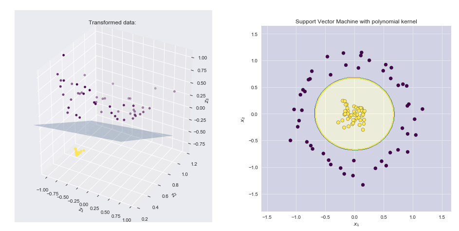
— Xavier Bourret SicotteFollowing the series on SVM, we will now explore the theory and intuition behind Kernels and Feature maps, showing the link between the two as well as advantages and disadvantages. The notebook is divided into two main sections: 1. Theory, derivations and pros and cons of the two concepts. 2. An intuitive and visual interpretation in 3 dimensions
 Tags:
Tags:
Support Vector Machine: Python implementation using CVXOPT
— Xavier Bourret SicotteIn this second notebook on SVMs we will walk through the implementation of both the hard margin and soft margin SVM algorithm in Python using the well known CVXOPT library. While the algorithm in its mathematical form is rather straightfoward, its implementation in matrix form using the CVXOPT API can be challenging at first. This notebook will show the steps required to derive the appropriate vectorized notation as well as the inputs needed for the API.
 Tags:
Tags:
Support Vector Machine: calculate coefficients manually
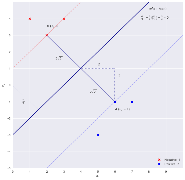
— Xavier Bourret SicotteIn this first notebook on the topic of Support Vector Machines, we will explore the intuition behind the weights and coefficients by solving a simple SVM problem by hand.
 Tags:
Tags:
Linear and Quadratic Discriminant Analysis
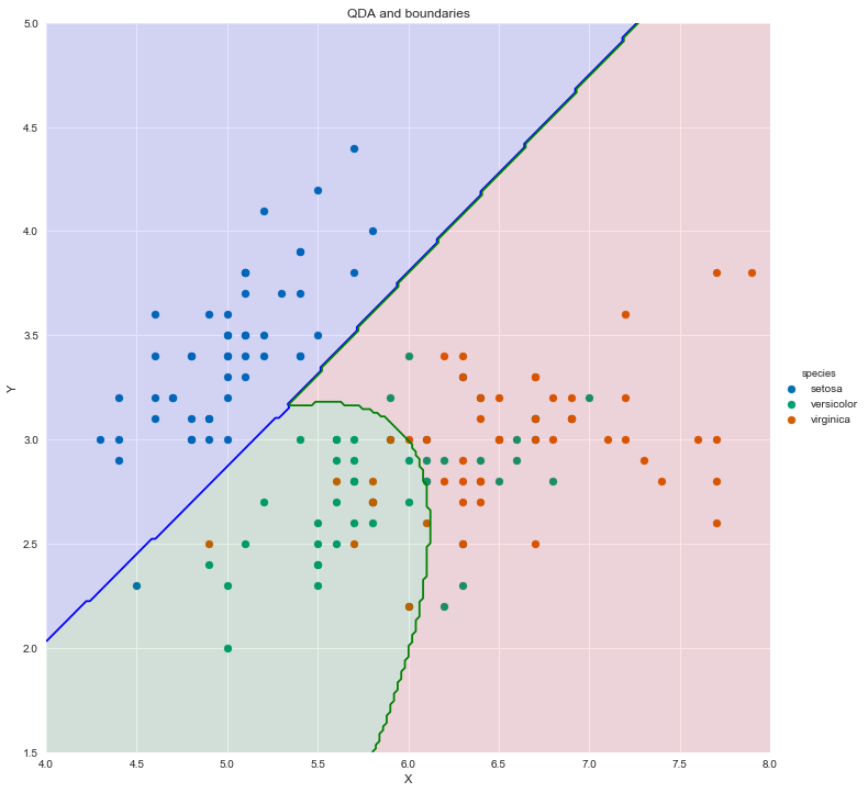
— Xavier Bourret SicotteExploring the theory and implementation behind two well known generative classification algorithms. Linear discriminative analysis (LDA) and Quadratic discriminative analysis (QDA). This notebook will use the Iris dataset as a case study for comparing and visualizing the prediction boundaries of the algorithms
 Tags:
Tags:
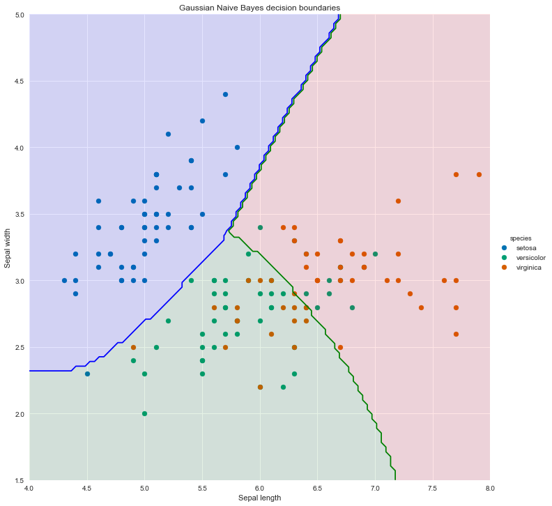
Gaussian Naive Bayes Classifier: Iris data set
— Xavier Bourret SicotteIn this short notebook, we will use the Iris dataset example and implement instead a Gaussian Naive Bayes classifier using Pandas, Numpy and Scipy.stats libraries. Results are then compared to the Sklearn implementation as a sanity check
 Tags:
Tags:
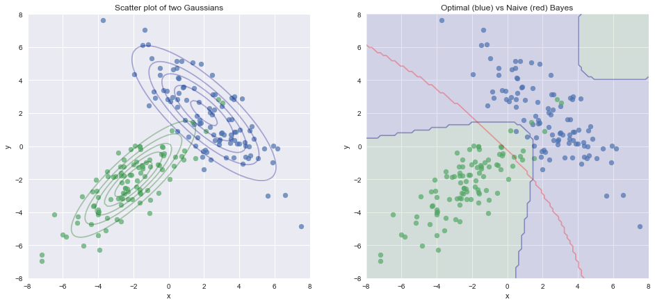
Optimal Bayes Classifier
— Xavier Bourret SicotteThis notebook summarises the theory and the derivation of the optimal bayes classifier. It then provides a comparison of the boundaries of the Optimal and Naive Bayes classifiers.
 Tags:
Tags:
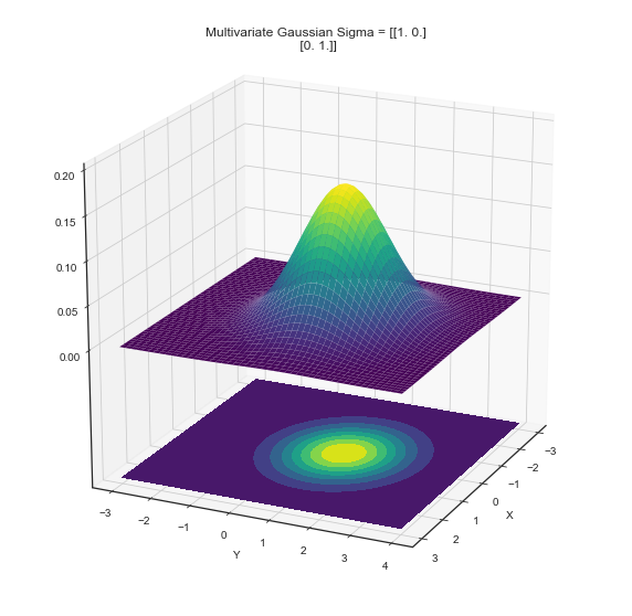
Maximum Likelihood Estimator: Multivariate Gaussian Distribution
— Xavier Bourret SicotteThe Multivariate Gaussian appears frequently in Machine Learning and this notebook aims to summarize the full derivation of its Maximum Likelihood Estimator
 Tags:
Tags:
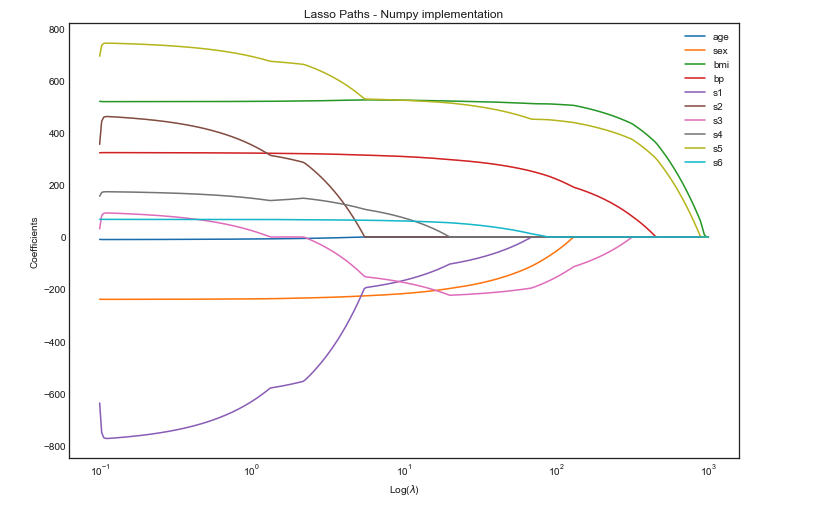
Lasso regression: implementation of coordinate descent
— Xavier Bourret SicotteFollowing the blog post where we have derived the closed form solution for lasso coordinate descent, we will now implement it in python numpy and visualize the path taken by the coefficients as a function of lambda. Our results are also compared to the Sklearn implementation as a sanity check.
 Tags:
Tags:
Ridge and Lasso: visualizing the optimal solutions
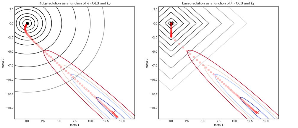
— Xavier Bourret SicotteThis short notebook offers a visual intuition behind the similarity and differences between Ridge and Lasso regression. In particular we will the contour of the Olrdinary Least Square (OLS) cost function, together with the L2 and L1 cost functions.
 Tags:
Tags:
Lasso regression: derivation of the coordinate descent update rule
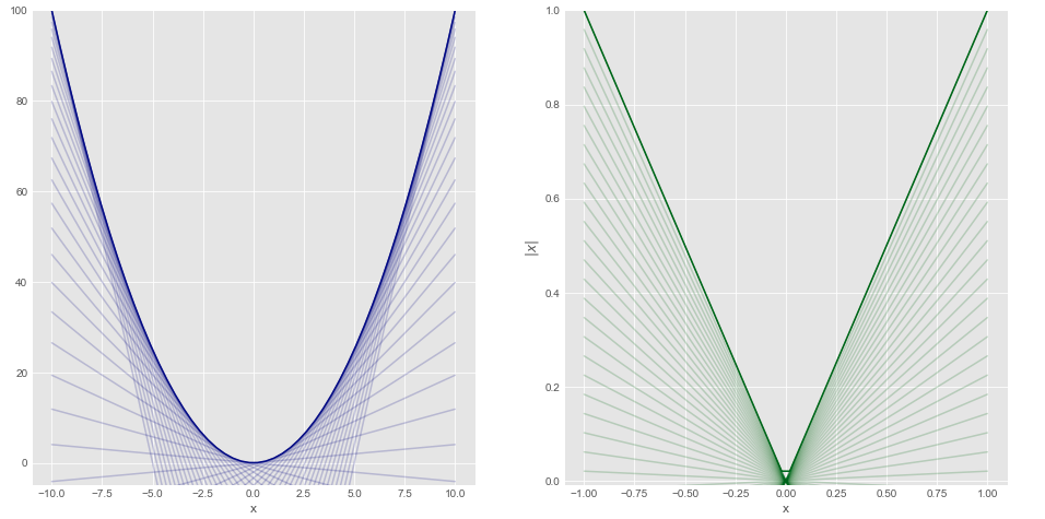
— Xavier Bourret SicotteThis post describes how to derive the solution to the Lasso regression problem when using coordinate gradient descent. It also provides intuition and a summary of the main properties of subdifferentials and subgradients. Code to generate the figure is in Python.
 Tags:
Tags:
Coordinate Descent - Implementation for linear regression
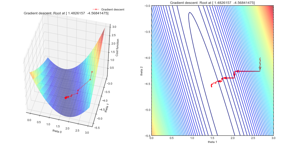
— Xavier Bourret SicotteDescription of the algorithm and derivation of the implementation of Coordinate descent for linear regression in Python. Visualization of the "staircase" steps using surface and contour plots as well as a simple animation. This implementation will serve as a step towards more complex use cases such as Lasso.
 Tags:
Tags:
Ridge regression and L2 regularization - Introduction
— Xavier Bourret SicotteThis notebook is the first of a series exploring regularization for linear regression, and in particular ridge and lasso regression. We will focus here on ridge regression with some notes on the background theory and mathematical derivations and python numpy implementation. Finally we will provide visualizations of the cost functions with and without regularization to help gain an intuition as to why ridge regression is a solution to poor conditioning and numerical stability.
 Tags:
Tags:
Choosing the optimal model: Subset selection
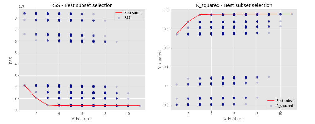
— Xavier Bourret SicotteIn this notebook we explore some methods for selecting subsets of predictors. These include best subset and stepwise selection procedures. Code and figures inspired from the book ISLR - chapter 6 - converted into python.
 Tags:
Tags:
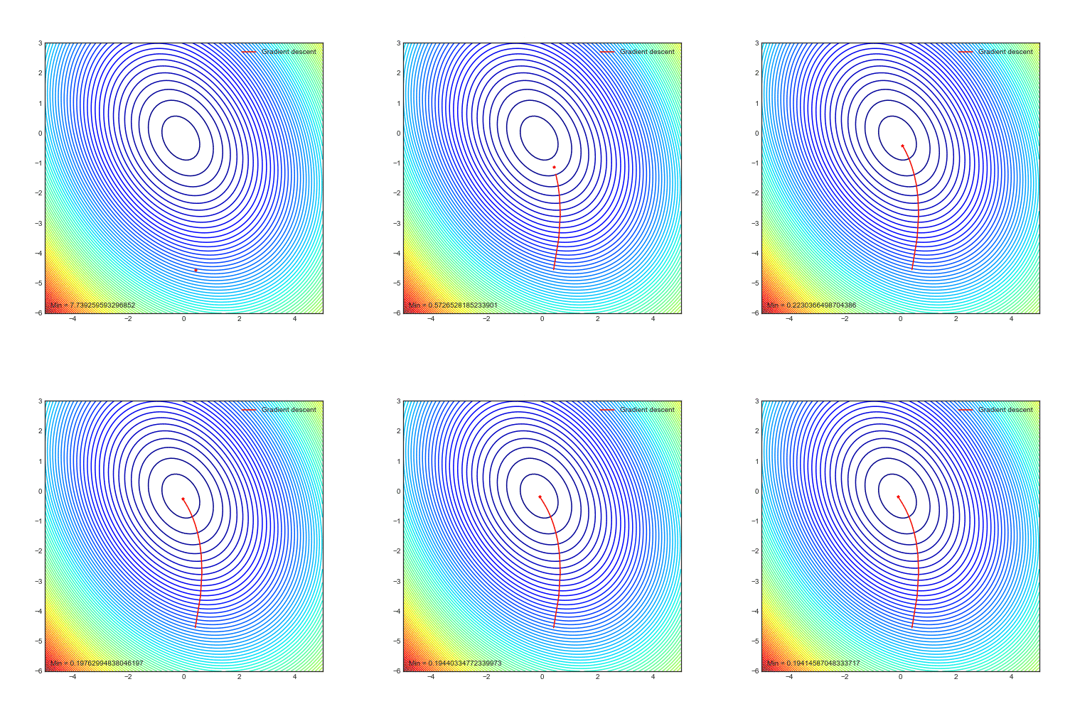
Animations of gradient descent: Ridge regression
— Xavier Bourret SicotteAnimation of gradient descent in Python using Matplotlib for contour and 3D plots. This particular example uses polynomial regression with ridge regularization
 Tags:
Tags:
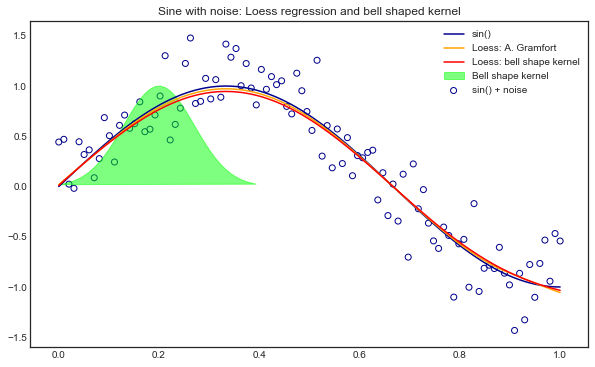
Locally Weighted Linear Regression (Loess)
— Xavier Bourret SicotteIntroduction, theory, mathematical derivation of a vectorized implementation of Loess regression. Comparison of different implementations in python and visualization of the result on a noisy sine wave
 Tags:
Tags:
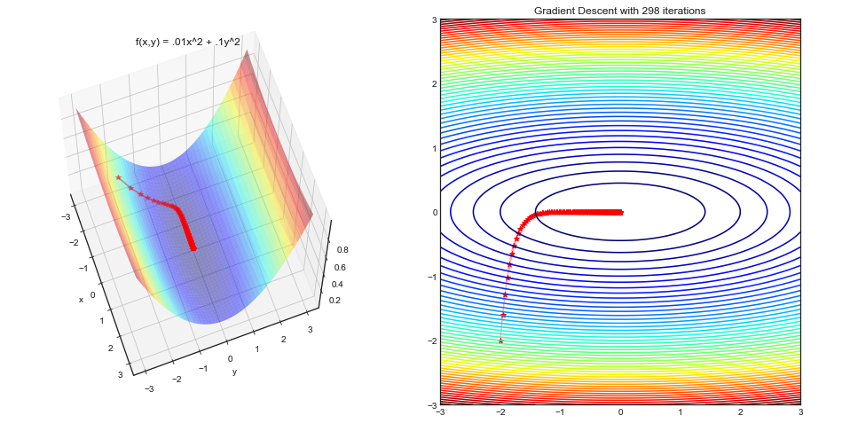
Introduction to Optimization and Visualizing algorithms
— Xavier Bourret SicotteIntroductory optimization algorithms implemented in Python Numpy and their corresponding visualizations using Matplotlib. A case study comparison between Gradient Descent and Newton's method using the Rosenbrock function.
 Tags:
Optimization
Visualization
Statistical inference on multiple linear regression
— Xavier Bourret SicotteStatistical inference on multiple linear regression in Python using Numpy, Statsmodel and Sklearn. Implementation of model selection, study of multicolinearity and residuals analysis.
 Tags:
statistics
regression
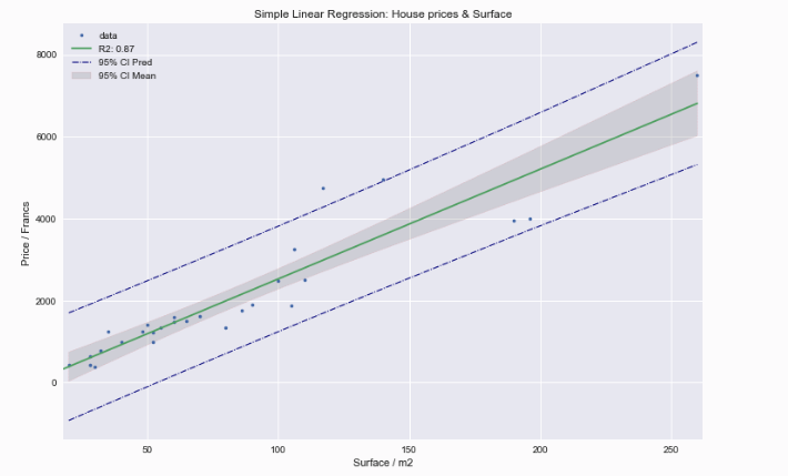
Statistical inference on simple linear regression
— Xavier Bourret SicotteImplementation of statistical inference in Python using Numpy, Statsmodel and Sklearn. Detailed breakdown of the formulae used and main assumptions behind the model. Some nice graphs on leverage and influence of observations.
 Tags:
statistics
regression